Dimensionality reduction-principal component analysis with Python
The dimensionality of a dataset refers to the number of variables and attributes the data possesses. High input variables datasets can affect the function and performance of the algorithm used. This problem is termed the curse of dimensionality.
To avoid this problem, it is necessary to reduce the number of input variables. Reduction of input features manifests in the reduction of dimensions of the feature space. This reduction is termed as dimensionality reduction, which refers to techniques that are used to reduce the features or dimensions in a dataset.
Why the need for dimensionality reduction?
The application of dimensionality reduction to a dataset gives the following benefits:
- Less storage space is needed as the dimensions are reduced
- Helps the algorithms function effectively
- Multicollinearity between redundant features is removed
- Visualization of data is much easier with fewer dimensions
- Overfitting of datasets is avoided
Methods of dimensionality reduction
Two methods are used when reducing dimensionality, and they are:
- Feature selection: the number of input variables are reduced in order to predict the target variables. Supervised and unsupervised techniques are the two main types of feature selection techniques. Supervised techniques can be further divided into wrapper, filter and embedded methods. Recursive feature elimination (RFE) is the method used under the wrapper technique. In the filter method, statistical methods are commonly used. The embedded technique makes use of decision trees method.
- Feature extraction: it is the process of extracting data from a complicated dataset to make up a new feature set. In feature extraction, the pre-existing input data has its dimensions reduced and each new variable is a linear or non-linear combination of the original input data. Principal component analysis, linear discriminant analysis (LDA) and ISOmetric feature MAPping (ISOMAP) are techniques used in feature extraction.
Dimensionality Reduction Techniques in Python
The following are some techniques of dimensionality reduction as applied in Python.
- Principal Component Analysis
- Missing Value Ratio
- Low Variance Filter
- High Correlation Filter
- Random Forest
Principal Component Analysis with Python
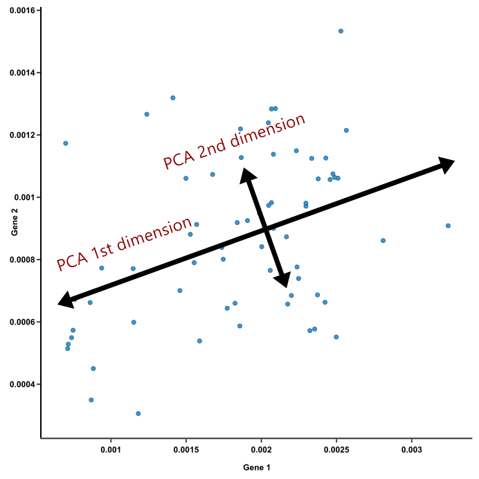
Principal Component Analysis (PCA) works on the principle of reducing the number of variables of a dataset while maintaining vital information relating to the dataset. Features or variables present in the original set are linearly combined. The resulting features from these combinations are termed principal components. The first principal component encapsulates the bulk of the variance present in the dataset. The second principal component takes the majority of the remaining variance in the dataset. This follows suite in the rest of the principal components. The principal components are not mutually related. Principal components are eigenvectors of a data’s covariance matrix. Eigenvectors are linear algebra concepts computed from the covariance matrix, which is a square matrix that calculates the covariance between each pair of elements of the initial variables. Every eigenvector has its corresponding eigenvalue and together, they sum up to the number of dimensions of the data. Eigenvalues are coefficients attached to eigenvectors which indicate the variance of each principal component.
Applications of Principal Component Analysis
The following are some applications of PCA:
- Data compression
- Time series prediction
- Image processing
- Pattern recognition
- Exploratory data analysis
- Visualization
Advantages and disadvantages of PCA
| Advantages | Disadvantages |
|---|---|
| 1. Correlated features are removed | 1. Difficult to interpret independent variables |
| 2. Algorithm performance is enhanced | 2. Data has to be standardized before PCA is done |
| 3. Reduces overfitting of data | 3. There might be loss of information |
| 4. Visualization of data is improved |
Figure 1 represents a figure of two principal components in a dataset:
#importing sklearn libraryimport sklearn#importing dataset from sklearn libraryimport sklearn.datasets as etheldatairis = etheldata.load_iris()from sklearn.decomposition import PCAimport matplotlib.pyplot as PCAplotfrom sklearn.model_selection import train_test_splitX, y = etheldata.load_iris(return_X_y=True)#scaling datafrom sklearn.preprocessing import StandardScalerX_scaler = StandardScaler () .fit_transform (X)X_scaler[:4]pca = PCA(n_components=3)pca.fit(X)X_tran = pca.transform(X)#visualization of outputfig, axe = PCAplot.subplots(dpi=400)axe.scatter(X_tran[:, 0], X_tran[:, 1], c=y, marker= 'o')fig.savefig("output/img.png")PCAplot.show(fig)
Other dimensionality reduction methods
- Missing Values Ratio: data columns with a ratio of missing values exceeding that of the standard are removed in this method. The rationale is that data columns with many missing values are less likely to contain useful information.
- Low variance filter: in this method, the data columns with a variance lower than a given threshold is removed. The variance is dependent on the column range so normalization is done before the filtering technique.
