How do subsequent convolution layers work?
Subsequent convolutional layers in convolutional neural networks (CNNs) work by extracting increasingly higher-level features of a given image.
CNNs are the go-to method when dealing with image data. CNNs work by detecting spatial features in an image through the convolution operation.
How convolution works
In a layer of CNN, we obtain the feature map of an input image by computing its dot product with a kernel in successive regions of the image, in a sliding window operation, as shown in the slides below:
The shape of the output of a convolution is given by the formula:
Here:
N = input dimension
K = kernel size
P = padding
S = stride
Expected output
After executing the code, we can expect the following output:
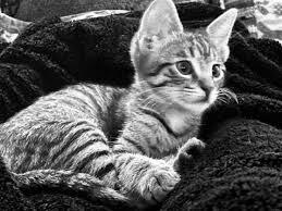
In the code below, we have provided an implementation of convolution from scratch in numpy. To run the code, you will have to upload an image on which the convolution operation can be applied. You can use your own image, or use the one provided here.
Note: You must upload a single channel grayscale image for the code to work properly.
Feel free to change the kernel and see how the convolution operation highlights different features with different kernels.
# Import the relevant librariesimport numpy as npfrom PIL import Image, ImageOpsimport matplotlib.pyplot as plt# Load the uploaded imageimg = Image.open('__ed_input.png')img = ImageOps.grayscale(img)img = img.resize(size=(448, 224))# Setup the relevant filters# 1. For image sharpeningsharpen = np.array([[0, -1, 0],[-1, 5, -1],[0, -1, 0]])# 2. For image blurringblur = np.array([[0.0625, 0.125, 0.0625],[0.125, 0.25, 0.125],[0.0625, 0.125, 0.0625]])# 3. For outliningoutline = np.array([[-1, -1, -1],[-1, 8, -1],[-1, -1, -1]])# An auxillary function to plot the original and transformed imagesdef plot_two_images(img1: np.array, img2: np.array):fig = plt.figure(figsize=(12, 12))fig.add_subplot(2, 1, 1)plt.imshow(img1, cmap='gray')plt.axis('off')plt.title("Original")fig.add_subplot(2, 1, 2)plt.imshow(img2, cmap='gray')plt.axis('off')plt.title("Transformed")plt.show()plt.savefig('./output/out.png')return# Determining output image size using the formula mentioned abovedef calculate_target_size(img_size: (int, int), kernel_size: int) -> int:out_x = (img_size[0]-kernel_size)+1out_y = (img_size[1]-kernel_size)+1return out_x, out_y# The convolution operationdef convolve(img: np.array, kernel: np.array) -> np.array:t_x_size, t_y_size = calculate_target_size(img_size=(img.shape[0], img.shape[1]),kernel_size=kernel.shape[0])k = kernel.shape[0]convolved_img = np.zeros(shape=(t_x_size, t_y_size))for i in range(t_x_size):for j in range(t_y_size):mat = img[i:i+k, j:j+k]convolved_img[i, j] = np.sum(np.multiply(mat, kernel))return convolved_img# Using the convolution operationimg_outlined = convolve(img=np.array(img), kernel=outline)# Plotting the imagesplot_two_images(img1=img,img2=img_outlined)
Explanation
Lines 2–4: We import the relevant libraries.
Lines 7–9: We load the uploaded image.
Lines 13–31: We declare a few kernels.
Lines 34–45: We define a function
plot_two_images()for plotting images.Lines 48–51: We define a function
calculate_target_size()to calculate output image sizes using the formula given above.Lines 54–67: We define the convolution operation function
convolve().Line 71: We call the
convolve()function for performing convolution.Lines 74–77: We call the
plot_two_images()function to plot the images.
Subsequent layers
The CNN is composed of multiple such convolutional layers. As we go deeper into a CNN, increasingly high-level features are extracted. For example, in facial recognition, the first layer detects edges. The next layer learns to detect parts of faces that are formed by those edges, such as eyelids. The next layers detect parts of faces, such as eyes, that are created by these features. The final layer identifies complete facial structures by combining various sub-level features such as eyes, nose, mouth, and ears.
During training, we attempt to learn these kernels by back-propagating the error in predicting the training dataset.
Free Resources
