Panorama Formation using OpenCV
Open Source Computer Vision (OpenCV) is an
Note: You can learn more about OpenCV.
Panorama
If we have two images that share similar features, stitching them from the overlapping region to make a panoramic view is possible. We can achieve this panoramic view using cv2 library in python. The provided code combines the images below:
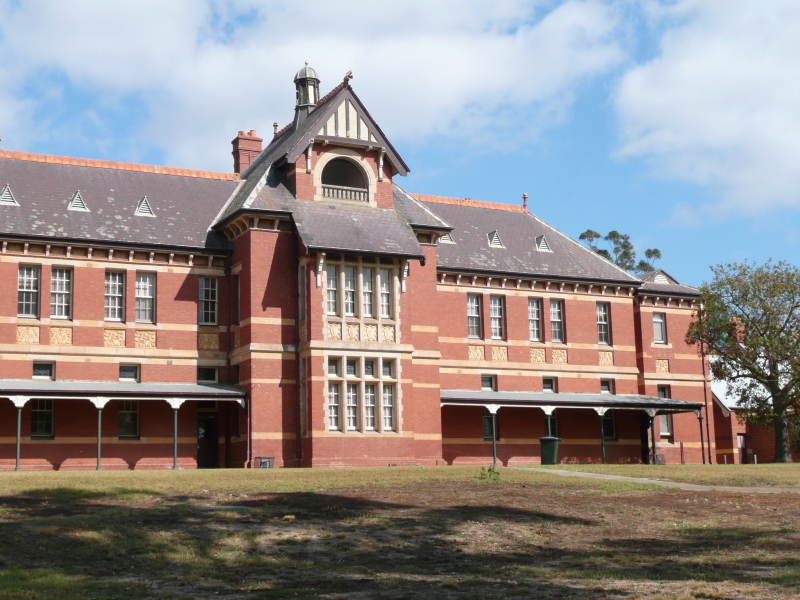
image1.jpg in the code)
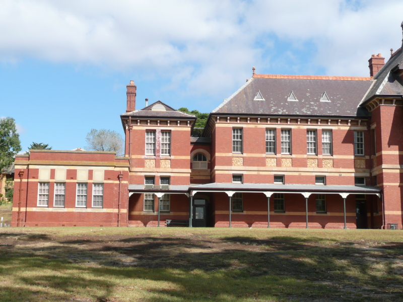
image2.jpg in the code)
The provided code stitches above two images and displays the resultant panorama as follows:


import numpy as np
import cv2
#Fnuction to resize the image to either (a x 720) or (720 x a)
def resizing(img):
    w=0
    h=0
    if(img.shape[1]>=img.shape[0]):
        target = img.shape[1]
        w = 720
        h = int(img.shape[0]/target*720)
    else:
        target = img.shape[0]
        h = 720
        w = int(w/target*720)
    img = cv2.resize(img,(w,h))
    return img

def image_stitching_function(img1,img2):
    #GrayScalling and resizing:-
    img1_greyScaled = resizing(cv2.cvtColor(img1,cv2.COLOR_BGR2GRAY)) #Greyscalling image
    img2_greyScaled = resizing(cv2.cvtColor(img2,cv2.COLOR_BGR2GRAY)) #Greyscalling image

    #Normalizing:-
    norm = np.zeros((800,800))
    img1_greyScaled_normalized = cv2.normalize(img1_greyScaled,norm,0,255,cv2.NORM_MINMAX)    #Normalizing image
    img2_greyScaled_normalized = cv2.normalize(img2_greyScaled,norm,0,255,cv2.NORM_MINMAX)    #Normalizing image

    #Applying SIFT descriptors:-
    SIFT_img1_greyScaled_normalized = cv2.SIFT_create()
    SIFT_img2_greyScaled_normalized = cv2.SIFT_create()

    #Detecting features:-
    (kps1, features1) = SIFT_img1_greyScaled_normalized.detectAndCompute(img1_greyScaled_normalized, None)
    kps2 = np.float32([kp.pt for kp in kps1]) #Making it numpy array of the key poitns
    (kps2, features2) = SIFT_img2_greyScaled_normalized.detectAndCompute(img2_greyScaled_normalized, None)
    kps2 = np.float32([kp.pt for kp in kps2]) #Making it numpy array of the key poitns

    #Matching keypoints
    matcher = cv2.DescriptorMatcher_create("BruteForce")
    rawMatches = matcher.knnMatch(features1,features2,2)  #k nearest neighbour key points
    matches = list()    #lists of matches
    M = None    #Tupple of (matches_list, homography_Matrix, Status)
    H = None
    for m in rawMatches:
        if len(m) == 2 and m[0].distance < m[1].distance * 0.3:
            matches.append((m[0].trainIdx,m[0].queryIdx))   #stroing nearest neighbours from overlapped region of the images
    if len(matches) > 4:    #We need atleast four points to get the Homography matrix
        # construct the two sets of points
        ptsA = np.float32([kps20[i] for (_, i) in matches])
        ptsB = np.float32([kps21[i] for (i, _) in matches])
        # compute the homography between the two sets of points
        (H, status) = cv2.findHomography(ptsB, ptsA, cv2.RANSAC,None)
        print("Homography matrix:",H)
        # return the matches, homograpy matrix and status of each matched point as a tuple of three in M.
        M = (matches, H, status)

    #Aplying Warping:-
    result = cv2.warpPerspective(img2_greyScaled_normalized,H,(img2_greyScaled_normalized.shape[1]+img1_greyScaled_normalized.shape[1], img2_greyScaled_normalized.shape[0]+40))
    #putting the source image over the destination image:-
    result[0:img1_greyScaled_normalized.shape[0],0:img1_greyScaled_normalized.shape[1]] = img1_greyScaled_normalized
    cv2.imshow("Final Result",result)   #showing the matching result
    cv2.waitKey(0)


def main():
    img1 = cv2.imread("image1.jpg")
    img2 = cv2.imread("image2.jpg")
    image_stitching_function(img2,img1)
main()
Code explanation
Lines 65–69: This is the
main()function receiving the images and then passing them to theimage_stitching_function()function which will then stitch both images and display the results.Lines 4–16: The function
resizing()takes an imageimgas a parameter and reshapes it to either aw x 720pixels or a720 x hpixel image usingresize()function (on line15) depending upon the image's aspect ratio. This helps the algorithm to stitch the images without getting into any anomaly.Lines 20–21: The images are grayscaled using the
cv2.cvtColor()function. The grayscaled images are then passed to theresizing()function for resizing. Grayscaling the images is important because it simplifies them and removes the influence of varying lighting conditions. Additionally, it facilitates easier feature detection.Lines 24–26: Grayscaled images are being normalized using
normalize()method ofcv2to a range of0to255. By normalizing the images, pixel values get scaled to a desired range making it easier to compare them.Lines 29–30: The code applies cv2's built-in SIFT detector to the normalized images to detect their invariant local features, regardless of their rotation, scale and lighting conditions.
Lines 33–36: The detecting features are now getting stored in the variables
feature20andfeature21, and the key points where the invariant features have been detected are getting stored inkps20andkps21for both images, respectively.Lines 39–40: The
cv2.DescriptorMatcher_create()method from thecv2library creates a matcher object that performs a "Brute Force" feature mapping. This mapping is stored in thematchervariable. Once the matcher is created, it applies the k-nearest neighbors (knn) algorithm using theknnMatch()method.Lines 41–55: All the matches are stored as
numpyarray in matches. If the number of matches exceeds4, the code calculates the homography matrixH. It selects the matched key points from both images (ptsAandptsB) and usesfindHomography()method ofcv2library with theRANSAC method It stands for Random Sample Consensus. It is a robust estimation algorithm to estimate the parameters of a mathematical model that best fits a given set of data points. M.Lines 58–62: After obtaining the homography matrix, it is applied to the images using the
warpPerspective()method from thecv2library. This process aligns the images based on the estimated transformation. Once the images are stitched together, the code displays the resulting stitched image. The code waits for the viewer (usingwaitKey()method) to press any key to stop displaying the image.
Note: Learn how to do dilation of an image using OpenCV.
Free Resources
