PyTorch tutorial: a quick guide for new learners

Python is well-established as the go-to language for data science and machine learning, partially thanks to the open-source ML library PyTorch.

PyTorch’s combination of powerful deep neural network building tools and ease-of-use make it a popular choice for data scientists. As its popularity grows, more and more companies are moving from TensorFlow to PyTorch, making now the best time to get started with PyTorch.

Today, we’ll help understand what makes PyTorch so popular, some basics of using PyTorch, and help you make your first computational models.

Here’s what we’ll cover today:

• What is PyTorch?
• Why use PyTorch?
• PyTorch Basics
• Computation Graphs with PyTorch
• Hands-on with PyTorch: Multi-path computation graph
• Next steps for your learning

Start building PyTorch projects in half the time

Learn to build and optimize PyTorch neural networks with hands-on practice.

Make Your First GAN Using PyTorch

What is PyTorch?#

PyTorch is an open-source machine learning Python library used for deep learning implementations like computer vision (using TorchVision) and natural language processing. It was developed by Facebook’s AI research lab (FAIR) in 2016 and has since been adopted across the fields of data science and ML.

PyTorch makes machine learning intuitive for those already familiar with Python and has great features like OOP support and dynamic computation graphs.

Along with building deep neural networks, PyTorch is also great for complicated mathematical computations because of its GPU acceleration. This feature allows PyTorch to use your computer’s GPU to massively speed up computations.

This combination of unique features and PyTorch’s unparalleled simplicity makes it one of the most popular deep learning libraries, only rivaled by TensorFlow for the top spot.

Why use PyTorch?#

Before PyTorch, developers used advanced calculus to find the relationships between back-propagated errors and node weighting. Deeper neural networks called for more and more complicated operations, which restricted machine learning in scale and approachability.

Now, we can use ML libraries to automatically complete calculus! ML libraries can compute any size or shape network in a matter of seconds, allowing more developers to build bigger and better networks.

PyTorch takes this accessibility one step further by behaving like standard Python. Further, you can use additional Python libraries with PyTorch, such as popular debuggers like the PyCharm debugger.

PyTorch vs. TensorFlow#

The main difference between PyTorch and TensorFlow is a tradeoff between simplicity and performance: PyTorch is easier to learn (especially for Python programmers), while TensorFlow has a learning curve but performs better and is more widely used.

• Popularity: TensorFlow is the current go-to tool for industry professionals and researchers because it was released 1 year earlier than PyTorch. However, PyTorch users are growing at a faster rate than TensorFlow, suggesting that PyTorch may soon be the most popular.

• Data parallelism: PyTorch includes declarative data parallelism, in other words it automatically spreads the workload of data processing across different GPUs to speed up performance. TensorFlow has parallelism, but it requires you to assign work manually, which is often time-consuming and less efficient.

• Dynamic vs. Static Graphs: PyTorch has dynamic graphs by default that respond to new data immediately. TensorFlow has limited support for dynamic graphs using TensorFlow Fold but mostly uses static graphs.

• Integrations: PyTorch is good to use for projects on AWS because of its close connection through TorchServe. TensorFlow is well integrated with Google Cloud and is suited for mobile applications due to its use of Swift API.

• Visualization: TensorFlow has more robust visualization tools and offers you finer control over graph settings. PyTorch’s Visdom visualization tool or other standard plotting libraries like matplotlib are not as fully featured as TensorFlow, but they’re easier to learn.

Enjoying the article? Scroll down to sign up for our free, bi-monthly newsletter.

PyTorch Basics#

Tensors#

PyTorch tensors are multidimensional array variables used as the foundation for all advanced operations. Unlike standard numeric types, tensors can be assigned to use either your CPU or GPU to speed up operations.

They’re similar to an n-dimensional NumPy array and can even be converted to a NumPy array in just a single line.

Tensors come in 5 types:

• FloatTensor: 32-bit float
• DoubleTensor: 64-bit float
• HalfTensor: 16-bit float
• IntTensor: 32-bit int
• LongTensor: 64-bit int

As with all numeric types, you want to use the smallest type that fits your needs to save memory. PyTorch uses FloatTensor as the default type for all tensors, but you can change this using

torch.set_default_tensor_type(t)

To initialize two FloatTensors:

import torch
# initializing tensors
a = torch.tensor(2)
b = torch.tensor(1)

Tensors can be used like other numeric types in simple mathematical operations.

# addition
print(a+b)
# subtraction
print(b-a)
# multiplication
print(a*b)
# division
print(a/b)

You can also move tensors to be handled by the GPU using cuda.

if torch.cuda.is_available():
    x = x.cuda()
    y = y.cuda()
    x + y

As tensors are matrices in PyTorch, you can set tensors to represent a table of numbers:

ones_tensor = torch.ones((2, 2)) # tensor containing all ones
rand_tensor = torch.rand((2, 2)) # tensor containing random values

Here, we’re specifying that our tensor should be a 2x2 square. The square is populated with either all ones when using the ones() function or random numbers when using the rand() function.

Neural Networks#

PyTorch is commonly used to build neural networks due to its exceptional classification models like image classification or convolutional neural networks (CNN).

Neural networks are layers of connected and weighted data nodes. Each layer allows the model to home in on which classification the input data most closely matches.

Neural networks are only as good as their training and therefore need big datasets and Generative Adversarial Networks (GANs), which generate more challenging training data based on those already mastered by the model.

PyTorch defines neural networks using the torch.nn package, which contains a set of modules to represent each layer of a network.

Each module receives input tensors and computes output tensors, which work together to create the network. The torch.nn package also defines loss functions that we use to train neural networks. The steps to building a neural network are:

• Construction: Create neural network layers, set up parameters, establish weights and biases.
• Forward Propagation: Calculate the predicted output using your parameters. Measure error by comparing predicted and actual output.
• Back-propagation: After finding the error, take the derivative of the error function in terms of the parameters of our neural network. Backward propagation allows us to update our weight parameters.
• Iterative Optimization: Minimize errors by using optimizers that update parameters through iteration using gradient descent.

Here’s an example of a neural network in PyTorch:

import torch
import torch.nn as nn
import torch.nn.functional as F
class Net(nn.Module):
    def __init__(self):
        super(Net, self).__init__()
        # 1 input image channel, 6 output channels, 3x3 square convolution
        # kernel
        self.conv1 = nn.Conv2d(1, 6, 3)
        self.conv2 = nn.Conv2d(6, 16, 3)
        # an affine operation: y = Wx + b
        self.fc1 = nn.Linear(16 * 6 * 6, 120)  # 6*6 from image dimension
        self.fc2 = nn.Linear(120, 84)
        self.fc3 = nn.Linear(84, 10)
    def forward(self, x):
        # Max pooling over a (2, 2) window
        x = F.max_pool2d(F.relu(self.conv1(x)), (2, 2))
        # If the size is a square you can only specify a single number
        x = F.max_pool2d(F.relu(self.conv2(x)), 2)
        x = x.view(-1, self.num_flat_features(x))
        x = F.relu(self.fc1(x))
        x = F.relu(self.fc2(x))
        x = self.fc3(x)
        return x
    def num_flat_features(self, x):
        size = x.size()[1:]  # all dimensions except the batch dimension
        num_features = 1
        for s in size:
            num_features *= s
        return num_features
net = Net()
print(net)

The nn.module designates that this will be a neural network then we define it with 2 conv2d layers, which perform a 2D convolution, and 3 linear layers, which perform linear transformations.

Next, we define a forward method to outline how to do forward propagation. We don’t need to define a backward propagation method because PyTorch includes a backwards() function by default.

Don’t worry if this seems confusing right now, we’ll cover simpler PyTorch implementations later in this tutorial.

Autograd#

Autograd is a PyTorch package used to calculate derivatives essential for neural network operations. These derivatives are called gradients. During a forward pass, autograd records all operations on a gradient-enabled tensor and creates an acyclic graph to find the relationship between the tensor and all operations. This operation collection is called automatic differentiation.

The leaves of this graph are input tensors, and the roots are output tensors. Autograd calculates the gradient by tracing the graph from the root to the leaf and multiplying every gradient in the way using the chain rule.

After calculating the gradient, the value of the derivative is automatically populated as a grad attribute of the tensor.

import torch
# pytorch tensor
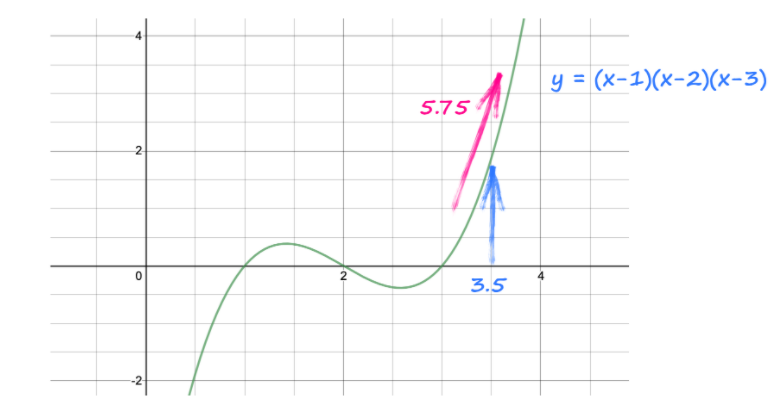
x = torch.tensor(3.5, requires_grad=True)
# y is defined as a function of x
y = (x-1) * (x-2) * (x-3)
# work out gradients
y.backward()

By default, requires_grad is set to false and PyTorch will not track gradients. Specifying requires_grad as True during initialization will make PyTorch track gradients for this particular tensor whenever we perform some operation on it.

This code looks at y and sees that it came from (x-1) * (x-2) * (x-3) and automatically works out the gradient $\frac{dy}{dx}$, $3x^2 - 12x + 11$

The instruction also works out the numerical value of that gradient and places it inside the tensor x alongside the actual value of x, 3.5.

All together, the gradient is 3 * (3.5 * 3.5) - 12 * (3.5) + 11 = 5.75.

Gradients accumulate by default, which could influence the result if not reset. Use model.zero_grad() to re-zero your graph after each gradient.

Optimizers#

Optimizers allow you to update the weights and biases within a model to reduce error. This allows you to edit how your model works without having to remake the whole thing.

All PyTorch optimizers are contained in the torch.optim package, with each optimization scheme designed to be useful in specific situations. The torch.optim module allows you to build an abstract optimization scheme by just passing a list of params. PyTorch has many optimizers to choose from, meaning there’s almost always one that best fits your needs.

For example, we can implement the common optimization algorithm, SGD (Stochastic Gradient Descent), to smooth our data.

import torch.optim as optim
params = torch.tensor([1.0, 0.0], requires_grad=True)
learning_rate = 1e-3
## SGD
optimizer = optim.SGD([params], lr=learning_rate)

After updating the model, use optimizer.step() to tell PyTorch to recalculate the model. Without using optimizers, we would need to manually update the model parameters one by one using a loop:

    for params in model.parameters(): 
       params -= params.grad * learning_rate

Overall, optimizers save a lot of time by allowing you to optimize your data weighting and alter your model without remaking it.

Computation Graphs with PyTorch#

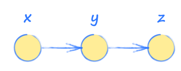
To better understand PyTorch and neural networks, it’s important to practice with computation graphs. These graphs are essentially a simplified version of neural networks with a sequence of operations used to see how the output of a system is affected by the input.

In other words, input x is used to find y, which is then used to find the output z.

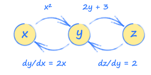
Imagine that y and z are calculated as follows:

$y = x^2$

$z = 2y + 3$

However, we’re interested in how how output z changes with input x, so we’ll need to do some calculus:

$\frac{dz}{dx} = \frac{dz}{dy}*\frac{dy}{dx}$

$\frac{dz}{dx} = 2.2x$

$\frac{dz}{dx} = 4x$

Using this, we can see that input x=3.5 will make z = 14.

Knowing how to define each tensor in terms of the others (y and z in terms of x, z in terms of y, etc.) allows PyTorch to build a picture of how these tensors are connected.

This picture is called a computation graph and can help us understand how PyTorch works behind the scenes.

Using this graph, we can see how each tensor will be affected by a change in any other tensor. These relationships are gradients and are used to update a neural network during training.

These graphs are much easier to do using PyTorch than by hand, so let’s try it now that we understand what’s happening behind the scenes.

import torch
# set up simple graph relating x, y and z
x = torch.tensor(3.5, requires_grad=True)
y = x*x
z = 2*y + 3
print("x: ", x)
print("y = x*x: ", y)
print("z= 2*y + 3: ", z)
# work out gradients
z.backward()
print("Working out gradients dz/dx")
# what is gradient at x = 3.5
print("Gradient at x = 3.5: ", x.grad)

This finds that z = 14 just as we found by hand above!

Hands-on with PyTorch: Multi-path computation graph#

Now that you’ve seen a computation graph with a single set of relationships, let’s try a more complex example.

First, define two tensors, a and b, to function as our inputs. Make sure to set requires_grad=True so we can make gradients down the line.

import torch
# set up simple graph relating x, y and z
a = torch.tensor(3.0, requires_grad=True)
b = torch.tensor(2.0, requires_grad=True)

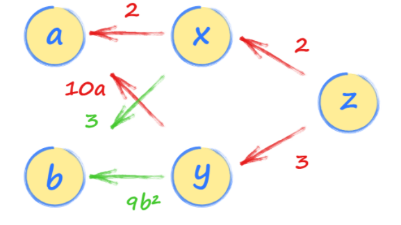
Next, set up the relationships between our input and each layer of our neural network, x, y, and z. Notice that z is defined in terms of x and y, while x and y are defined using our input values a and b.

import torch
# set up simple graph relating x, y and z
a = torch.tensor(3.0, requires_grad=True)
b = torch.tensor(2.0, requires_grad=True)

x = 2*a + 3*b
y = 5*a*a + 3*b*b*b
z = 2*x + 3*y

This builds a chain of relationships that PyTorch can follow to understand all the relationships between data.

We can now work out the gradient $\frac{dz}{da}$​​ by following the path back from z to a.

There are two paths, one going through x and the other through y. You should follow them both and add the expressions from both paths together. This makes sense because both paths from a to z contribute to the value of z.

We’d have found the same result if we had worked out $\frac{dz}{da}$ using the chain rule of calculus.

The first path through x gives us $2 * 2$ and the second path through y gives us $3 * 10a$. So, the rate at which z changes with $a$ is $4 + 30a$.

If a is 2, then $\frac{dz}{da}$​​ is $4+30∗2=64$.

We can confirm this in PyTorch by adding a backward propagation from z then asking for the gradient (or derivative) of a.

import torch
# set up simple graph relating x, y and z
a = torch.tensor(2.0, requires_grad=True)
b = torch.tensor(1.0, requires_grad=True)
x = 2*a + 3*b
y = 5*a*a + 3*b*b*b
z = 2*x + 3*y
print("a: ", a)
print("b: ", b)
print("x: ", x)
print("y: ", y)
print("z: ", z)
# work out gradients
z.backward()
print("Working out gradient dz/da")
# what is gradient at a = 2.0
print("Gradient at a=2.0:", a.grad)

Next steps for your learning#

Congratulations, you’ve now completed your quick start to PyTorch and Neural Networks. Completing a computational graph is an essential part of understanding deep learning networks.

As you learn advanced deep learning skills and applications, you’ll want to explore:

• Complex neural networks with optimization
• Visualization design
• Training with GANs

To help you get comfortable with real-world deep learning projects, Educative has made Make Your First GAN Using PyTorch. This course gives you a crash course in creating Generative Adversarial Networks (GANs) with PyTorch and explores how to build more effective, sophisticated GANs fit for professional use.

By the end, you’ll have the hands-on GAN practice needed to implement them in your own machine learning projects.

Happy learning!

Continue reading about deep learning and Python#

• Data Analysis Made Simple: Python Pandas Tutorial
• What is Deep Learning? A Tutorial for Beginners
• Scikit-learn Tutorial: how to implement linear regression